Triangle Boolean Subtraction
Introduction
In game development, navigation meshes are useful for defining walkable areas where AI characters can move. These meshes are made up of interconnected polygons that represent navigable surfaces, allowing for efficient pathfinding. My game uses navigation meshes for AI and player movement control. The need to handle dynamic obstacles was the main reason I developed this algorithm. The algorithm subtracts two triangles by removing the overlapping part from one of the triangles.
Here is an example:
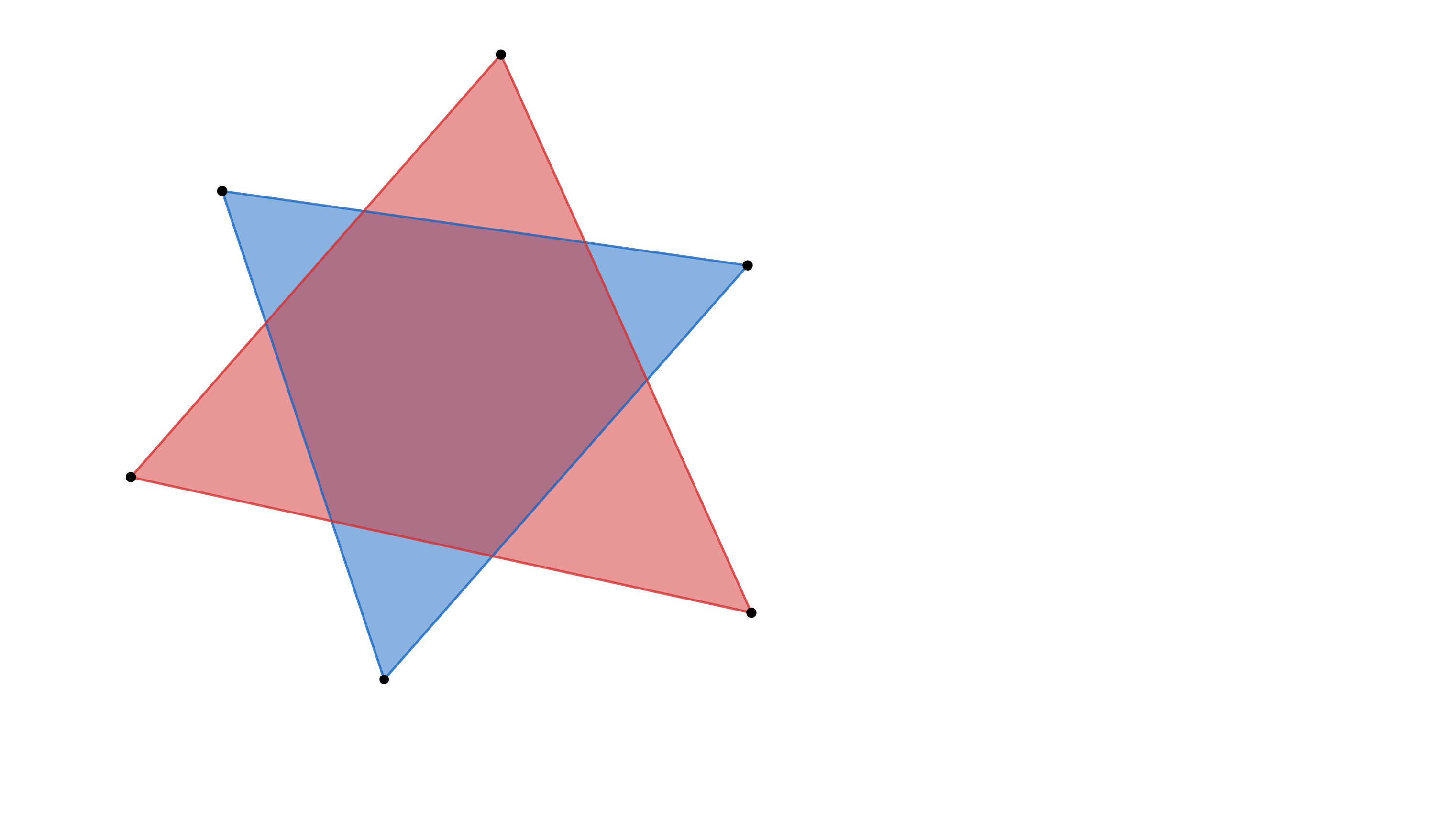
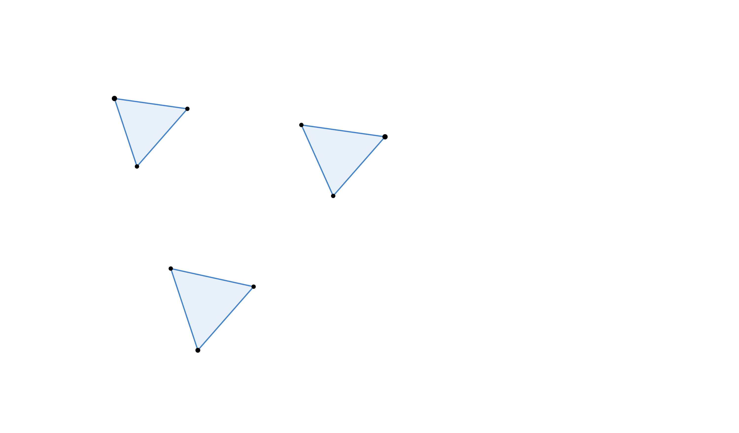
To create an obstacle on a navigation mesh, we need to mark the walkable area as unwalkable, which literally involves making a hole in the navigation polygon.
Initially, I researched existing algorithms that could perform this task, but I couldn’t find any ready-to-use solutions. However, I did find a detailed documentation that outlines how to construct such an algorithm, which you can check out here.
Using this as a foundation, I started building the algorithm. After some tests on various polygon types and the decision to use single precision floating point, the algorithm began to show issues — sometimes crashing, other times producing incorrect results.
To simplify the task, I decided to perform the subtraction on triangles, reducing the possible cases to 20. From here, I began developing the algorithm based on JE Wilson's guidelines.
For those who just want to see or use the code without reading through the whole explanation, here’s the GitHub link.
Implementation
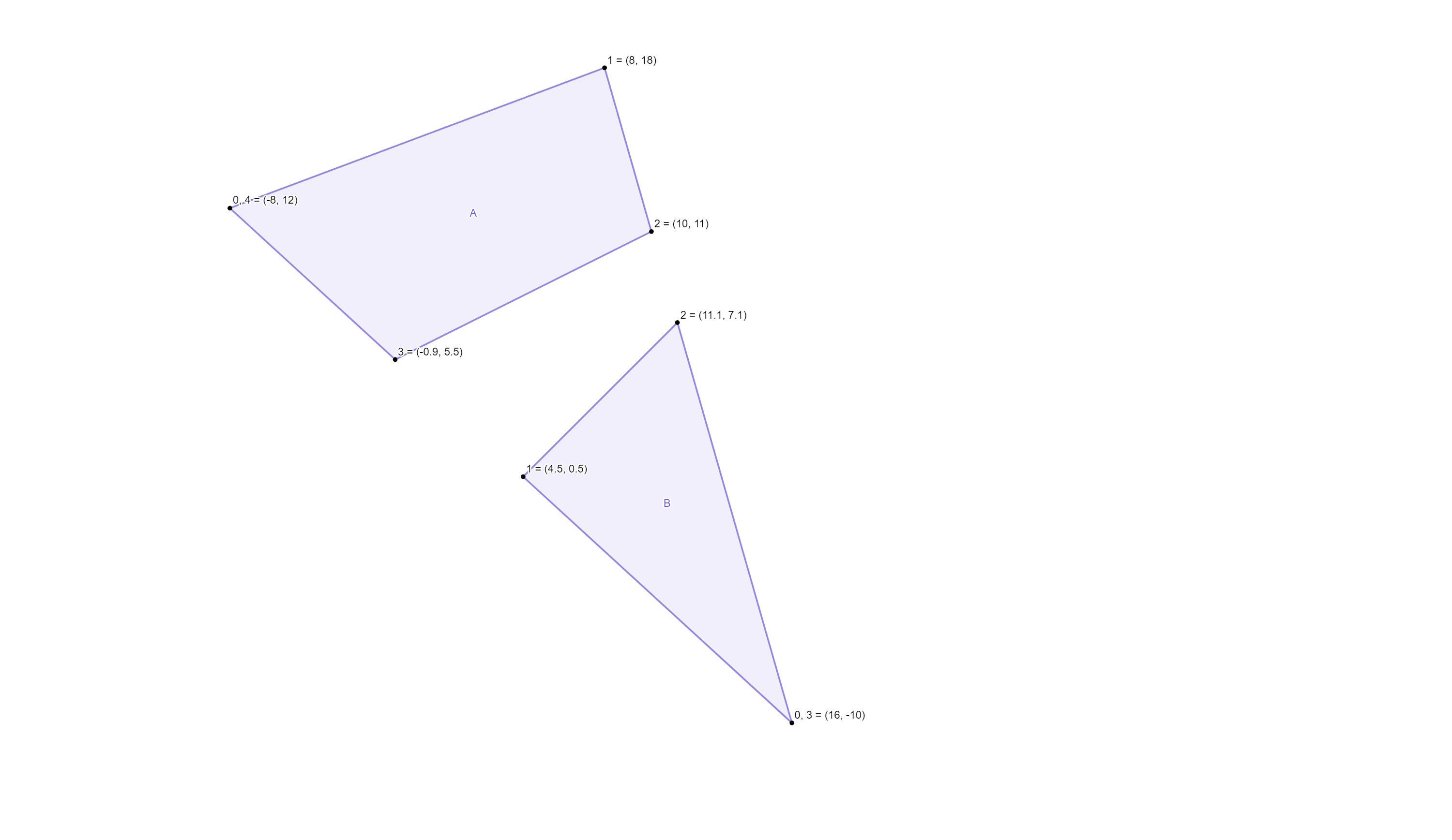
The image below will appear throughout the implementation steps to illustrate how it changes.
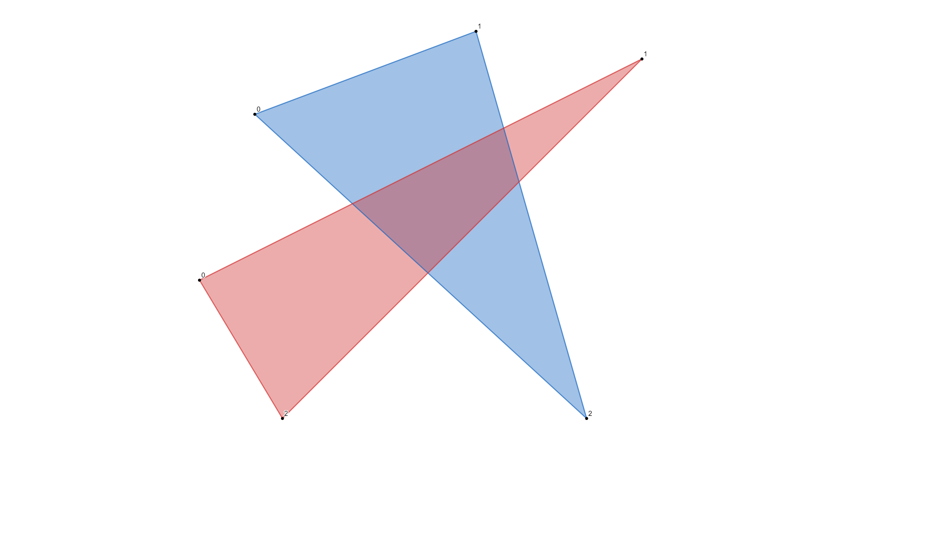
The first step is to check if two triangles overlap, excluding edges and vertices. For this, I used the Separating Axis Theorem (SAT). Then, I corrected the triangles’ orientation. The JE Wilson suggests calculating an offset based on the polygons’ orientation, but for simplicity, I made the algorithm work only on clockwise triangles. If necessary, the triangles are reoriented by swapping the second and last vertices. The orientation changes or calculationg an offset are needed for the later processing when from bunch of tables the resulting polygons will be constructed.
Next, I checked for triangle collinearity to eliminate cases with sliver triangles. If all checks pass, we create a polygon to hold points from the Subject triangle, allowing for the insertion of additional points if needed. The overlap polygon is then calculated using the Sutherland-Hodgman algorithm for clipping.

Once the Subtractor is created, it should be cleaned up by removing duplicate points and merging those that are very close together. We then check if the Subtractor's area is significant enough and if the difference between the Subtractor's area and the Subject's area is sufficient to proceed.
We then check if any vertex of the Subtractor lies on the first vertex of the Subject. If so, the points of the Subject are rotated clockwise in the array to avoid stacking too many points in one place and ensure the algorithm functions correctly. The first vertices of both the Subject and Subtractor are duplicated to their respective ends.
Next, we identify all points of the Subject that lie outside the Subtractor. This is straightforward, as points not found in the Subtractor are considered outside. We then determine which points of the Subtractor are on the Subject's edges and which edges they belong to. The result is a sorted array of points and a table detailing how many points are on each Subject edge. If no intersection points are found, we record the Subtractor as a hole in the Subject and exit the function.
Here are two function that perform operation above
internal points_between *
GetIntersectionPointsF32(polygon2 *A, polygon2 *B, v2 *OutputPoints, s32 *OutputCount, memory_arena *Arena)
{
    points_between *Result = PushArray(Arena, 3, points_between);

    temporary_memory TempMem = BeginTemporaryMemory(Arena);
    s32 TempCount = 0;
    v2 *Temp = PushArray(TempMem.Arena, SUBTRACTION_MAX_POINTS_PER_POLYGON, v2);

    for(s32 I = 0;
        I < A->VertexCount;
        ++I)
    {
        v2 Prv = A->Vertices[I];
        v2 Cur = A->Vertices[(I + 1) % A->VertexCount];
        if(!PointsAreEqualF32(Prv, Cur))
        {
            IntersectLineSegmentF32(B, Prv, Cur, Temp, &TempCount, Arena);
            s32 AddedCount = 0;
            for(s32 J = 0;
                J < TempCount;
                ++J)
            {
                if(IsNewPointF32(OutputPoints, *OutputCount, Temp[J]))
                {
                    OutputPoints[(*OutputCount)++] = Temp[J];
                    ++AddedCount;
                }
            }

            Result[I].Count = AddedCount;
            Result[I].I0 = I;
            Result[I].I1 = (I + 1) % A->VertexCount;

            TempCount = 0;
        }
    }

    EndTemporaryMemory(TempMem);

    return(Result);
}

internal b32
IntersectLineSegmentF32(polygon2 *A, v2 p1, v2 p2, v2 *Points, s32 *PointCount, memory_arena *Arena)
{
    temporary_memory TempMem = BeginTemporaryMemory(Arena);

    b32 Intersect = false;
    s32 TempPointCount = 0;
    v2 *TempPoints = PushArray(TempMem.Arena, SUBTRACTION_MAX_POINTS_PER_POLYGON, v2);

    for(s32 I = 0;
        I < (A->VertexCount - 1);
        ++I)
    {
        s32 J = (I + 1) % (A->VertexCount - 1);
        v2 p3 = A->Vertices[I];
        v2 p4 = A->Vertices[J];

        b32 Ends = false;
        if(DistanceToSegmentF32(p3, p1, p2) < SUBTRACT_DISTANCE_TO_EPSILON_F32)
        {
            TempPoints[TempPointCount++] = p3;
            Intersect = true;
            Ends = true;
        }

        if(DistanceToSegmentF32(p4, p1, p2) < SUBTRACT_DISTANCE_TO_EPSILON_F32)
        {
            TempPoints[TempPointCount++] = p4;
            Intersect = true;
            Ends = true;
        }
    }

    if(TempPointCount > 0)
    {
        ZeroArray((*PointCount)*sizeof(v2), Points);
        if(TempPointCount == 1)
        {
            Points[(*PointCount)++] = TempPoints[0];
        }
        else
        {
            s32 SortCount = TempPointCount;
            sort_entry *SortArray = PushArray(TempMem.Arena, TempPointCount, sort_entry);
            sort_entry *Temp = PushArray(TempMem.Arena, TempPointCount, sort_entry);
            for(s32 I = 0;
                I < TempPointCount;
                ++I)
            {
                sort_entry *Entry = SortArray + I;
                Entry->Index = I;
                Entry->SortKey = Length(p1 - TempPoints[I]);
            }

            RadixSort(SortCount, SortArray, Temp);

            v2 Last = TempPoints[SortArray[0].Index];
            Points[(*PointCount)++] = Last;
            for(s32 I = 1;
                I < TempPointCount;
                ++I)
            {
                v2 This = TempPoints[SortArray[I].Index];
                if(!PointsAreEqualF32(This, Last))
                {
                    Points[(*PointCount)++] = This;
                    Last = This;
                }
            }
        }
    }

    EndTemporaryMemory(TempMem);

    return(Intersect);
}
For the example illustrated above, the table will look like this:
| Edge Start Index | Edge End Index | Point Count |
|---|---|---|
| 0 | 1 | 0 |
| 1 | 2 | 2 |
| 2 | 3 | 2 |
If points are found, they are inserted into the Subject in the places described by the resulting table. We then need to build more tables, one for the Subject and one for the Subtractor. These tables contain information about each vertex of each polygon—whether the point is outside, if it is a crossing point, which point it crosses, a processed flag, and the point itself.
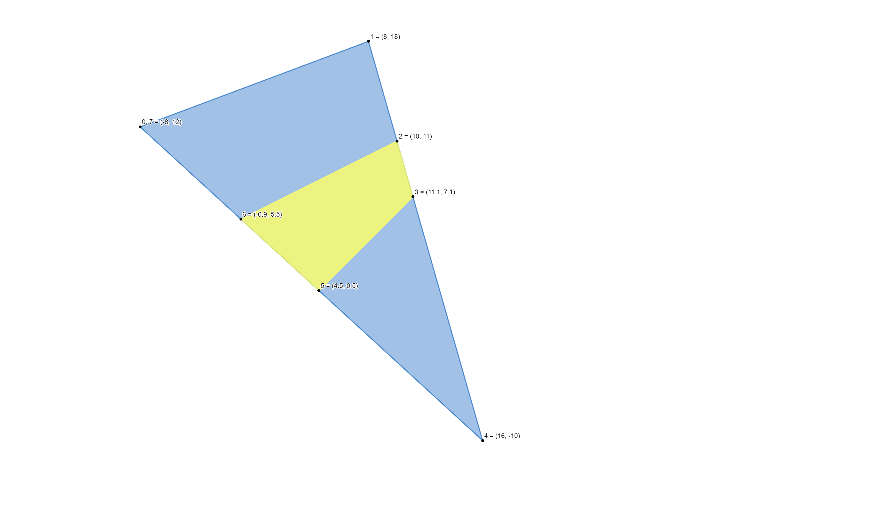
As a result, we have two tables that look like this:
Subject Vertex Info
| Vertex Index | Point (x, y) | Outside Flag | Cross | Processed Flag |
|---|---|---|---|---|
| 0 | (-8, 12) | true | -1 | false |
| 1 | (8, 18) | true | -1 | false |
| 2 | (10, 11) | false | 1 | false |
| 3 | (11.1, 7.1) | false | 2 | false |
| 4 | (16, -10) | true | -1 | false |
| 5 | (4.5, 0.5) | false | 3 | false |
| 6 | (-0.9, 5.5) | false | 4 | false |
| 7 | (-8, 12) | true | -1 | false |
Subtractor Vertex Info
| Vertex Index | Point (x, y) | Outside Flag | Cross | Processed Flag |
|---|---|---|---|---|
| 0 | (-0.9, 5.5) | false | 6 | false |
| 1 | (10, 11) | false | 2 | false |
| 2 | (11.1, 7.1) | false | 3 | false |
| 3 | (4.5, 0.5) | false | 5 | false |
| 4 | (-0.9, 5.5) | false | 6 | false |
With these tables built, the function that creates the resulting polygons is run, and the process is finished. The function that constructs the polygons is similar to the one described in the documentation, with a few modifications, so feel free to read through the implementation steps in section 2.5 here.
The result of this fucntion you can see below:
Why Single Precision Floating Point?
The initial implementation used double precision floating point, which has its advantages—fewer checks are needed, and results are more accurate for very small triangles. However, because this function will be used in a game, speed is crucial. Comparing the worst cases of both implementations, the single precision version is 2-2.5 times faster.
In benchmarks, the double-precision implementation consumes around 250,000 CPU cycles per frame in debug mode, while the single-precision version uses about 100,000 cycles. Additionally, the double precision requires twice as much memory as the single precision.
What is the Caveat?
The expected issue with the single precision implementation was incorrect handling of cases where Subtractor vertices or edges are very close to Subject vertices or edges. I addressed this by using EPSILON and merging points that are very close together, though finding the correct EPSILON value took some time.
Conclusion
The algorithm now works efficiently and quickly, though there’s always room for improvement. I tested the algorithm by generating overlapping triangles across all 20 cases, testing 2,048 cases per frame, which translates to about 7.4 billion cases per hour. After several hours of testing, no cases crashed, which I believe confirms the algorithm’s reliability.
That’s it for this post. If you want to implement your own algorithm, the documentation I used is quite helpful—much of the code comes directly from there. Otherwise, you can check out my repo with the source code of the implementation described.
Take care, BabyKaban
Enjoy Reading This Article?
Here are some more articles you might like to read next: